
Coronal loop
This article needs additional citations for verification. (March 2022) |

In solar physics, a coronal loop is a well-defined arch-like structure in the Sun's atmosphere made up of relatively dense plasma confined and isolated from the surrounding medium by magnetic flux tubes. Coronal loops begin and end at two footpoints on the photosphere and project into the transition region and lower corona. They typically form and dissipate over periods of seconds to days[1] and may span anywhere from 1 to 1,000 megametres (621 to 621,000 mi) in length.[2]
Coronal loops are often associated with the strong magnetic fields located within active regions and sunspots. The number of coronal loops varies with the 11 year solar cycle.
Origin and physical features
Due to a natural process called the solar dynamo driven by heat produced in the Sun's core, convective motion of the electrically conductive plasma which makes up the Sun creates electric currents, which in turn create powerful magnetic fields in the Sun's interior. These magnetic fields are in the form of closed loops of magnetic flux, which are twisted and tangled by solar differential rotation (the different rotation rates of the plasma at different latitudes of the solar sphere). A coronal loop occurs when a curved arc of the magnetic field projects through the visible surface of the Sun, the photosphere, protruding into the solar atmosphere.
Within a coronal loop, the paths of the moving electrically charged particles which make up its plasma—electrons and ions—are sharply bent by the Lorentz force when moving transverse to the loop's magnetic field. As a result, they can only move freely parallel to the magnetic field lines, tending to spiral around these lines. Thus, the plasma within a coronal loop cannot escape sideways out of the loop and can only flow along its length. This is known as the frozen-in condition.[3]
The strong interaction of the magnetic field with the dense plasma on and below the Sun's surface tends to tie the magnetic field lines to the motion of the Sun's plasma; thus, the two footpoints (the location where the loop enters the photosphere) are anchored to and rotate with the Sun's surface. Within each footpoint, the strong magnetic flux tends to inhibit the convection currents which carry hot plasma from the Sun's interior to the surface, so the footpoints are often (but not always) cooler than the surrounding photosphere. These appear as dark spots on the Sun's surface, known as sunspots. Thus, sunspots tend to occur under coronal loops, and tend to come in pairs of opposite magnetic polarity; a point where the magnetic field loop emerges from the photosphere is a North magnetic pole, and the other where the loop enters the surface again is a South magnetic pole.
Coronal loops form in a wide range of sizes, from 10 km to 10,000 km. Coronal loops have a wide variety of temperatures along their lengths. Loops at temperatures below 1 megakelvin (MK) are generally known as cool loops; those existing at around 1 MK are known as warm loops; and those beyond 1 MK are known as hot loops. Naturally, these different categories radiate at different wavelengths.[4]
A related phenomenon is the open flux tube, in which magnetic fields extend from the surface far into the corona and heliosphere; these are the source of the Sun's large scale magnetic field (magnetosphere) and the solar wind.
-
 A diagram showing the evolution of the solar magnetic flux over one solar cycle
 -
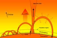 Diagram of the low corona and transition region, where many scales of coronal loops can be observed
 -
 A modelled example of a quiescent coronal loop (energy contributions)


Location
Coronal loops have been shown on both active and quiet regions of the solar surface. Active regions on the solar surface take up small areas but produce the majority of activity and are often the source of flares and coronal mass ejections due to the intense magnetic field present. Active regions produce 82% of the total coronal heating energy.[5][6]
Dynamic flows
Many solar observation missions have observed strong plasma flows and highly dynamic processes in coronal loops. For example, SUMER observations suggest flow velocities of 5–16 km/s in the solar disk, and other joint SUMER/TRACE observations detect flows of 15–40 km/s.[7][8] Very high plasma velocities (in the range of 40–60 km/s) have been detected by the Flat Crystal Spectrometer (FCS) on board the Solar Maximum Mission.
History of observations
Before 1991
Despite progress made by ground-based telescopes and eclipse observations of the corona, space-based observations became necessary to escape the obscuring effect of the Earth's atmosphere. Rocket missions such as the Aerobee flights and Skylark rockets successfully measured solar extreme ultraviolet (EUV) and X-ray emissions. However, these rocket missions were limited in lifetime and payload. Later, satellites such as the Orbiting Solar Observatory series (OSO-1 to OSO-8), Skylab, and the Solar Maximum Mission (the first observatory to last the majority of a solar cycle: from 1980 to 1989) were able to gain far more data across a much wider range of emission.[9][10]
1991–present day

In August 1991, the solar observatory spacecraft Yohkoh launched from the Kagoshima Space Center. During its 10 years of operation, it revolutionized X-ray observations. Yohkoh carried four instruments; of particular interest is the SXT instrument, which observed X-ray-emitting coronal loops. This instrument observed X-rays in the 0.25–4.0 keV range, resolving solar features to 2.5 arc seconds with a temporal resolution of 0.5–2 seconds. SXT was sensitive to plasma in the 2–4 MK temperature range, making its data ideal for comparison with data later collected by TRACE of coronal loops radiating in the extra ultraviolet (EUV) wavelengths.[11]
The next major step in solar physics came in December 1995, with the launch of the Solar and Heliospheric Observatory (SOHO) from Cape Canaveral Air Force Station. SOHO originally had an operational lifetime of two years. The mission was extended to March 2007 due to its resounding success, allowing SOHO to observe a complete 11-year solar cycle. SOHO has 12 instruments on board, all of which are used to study the transition region and corona. In particular, the Extreme ultraviolet Imaging Telescope (EIT) instrument is used extensively in coronal loop observations. EIT images the transition region through to the inner corona by using four band passes—171 Å FeIX, 195 Å FeXII, 284 Å FeXV, and 304 Å HeII, each corresponding to different EUV temperatures—to probe the chromospheric network to the lower corona.
In April 1998, the Transition Region and Coronal Explorer (TRACE) was launched from Vandenberg Air Force Base. Its observations of the transition region and lower corona, made in conjunction with SOHO, give an unprecedented view of the solar environment during the rising phase of the solar maximum, an active phase in the solar cycle. Due to the high spatial (1 arc second) and temporal resolution (1–5 seconds), TRACE has been able to capture highly detailed images of coronal structures, whilst SOHO provides the global (lower resolution) picture of the Sun. This campaign demonstrates the observatory's ability to track the evolution of steady-state (or 'quiescent') coronal loops. TRACE uses filters sensitive to various types of electromagnetic radiation; in particular, the 171 Å, 195 Å, and 284 Å band passes are sensitive to the radiation emitted by quiescent coronal loops.
See also
References
- ^ Loff, Sarah (2015-04-17). "Coronal Loops in an Active Region of the Sun". NASA. Retrieved 2022-03-28.
- ^ Reale, Fabio (July 2014). "Coronal Loops: Observations and Modeling of Confined Plasma" (PDF). Living Reviews in Solar Physics. 11 (4): 4. Bibcode:2014LRSP...11....4R. doi:10.12942/lrsp-2014-4. PMC 4841190. PMID 27194957. Retrieved 16 March 2022.
- ^ Malanushenko, A.; Cheung, M. C. M.; DeForest, C. E.; Klimchuk, J. A.; Rempel, M. (1 March 2022). "The Coronal Veil". The Astrophysical Journal. 927 (1): 1. arXiv:2106.14877. Bibcode:2022ApJ...927....1M. doi:10.3847/1538-4357/ac3df9. S2CID 235658491.
- ^ Vourlidas, A.; J. A. Klimchuk; C. M. Korendyke; T. D. Tarbell; B. N. Handy (2001). "On the correlation between coronal and lower transition region structures at arcsecond scales". Astrophysical Journal. 563 (1): 374–380. Bibcode:2001ApJ...563..374V. CiteSeerX 10.1.1.512.1861. doi:10.1086/323835. S2CID 53124376.
- ^ Aschwanden, M. J. (2001). "An evaluation of coronal heating models for Active Regions based on Yohkoh, SOHO, and TRACE observations". Astrophysical Journal. 560 (2): 1035–1044. Bibcode:2001ApJ...560.1035A. doi:10.1086/323064. S2CID 121226839.
- ^ Aschwanden, M. J. (2004). Physics of the Solar Corona. An Introduction. Praxis Publishing Ltd. ISBN 978-3-540-22321-4.
- ^ Spadaro, D.; A. C. Lanzafame; L. Consoli; E. Marsch; D. H. Brooks; J. Lang (2000). "Structure and dynamics of an active region loop system observed on the solar disc with SUMER on SOHO". Astronomy & Astrophysics. 359: 716–728. Bibcode:2000A&A...359..716S.
- ^ Winebarger, A. R.; H. Warren; A. van Ballegooijen; E. E. DeLuca; L. Golub (2002). "Steady flows detected in extreme-ultraviolet loops". Astrophysical Journal Letters. 567 (1): L89 – L92. Bibcode:2002ApJ...567L..89W. doi:10.1086/339796.
- ^ Vaiana, G. S.; J. M. Davis; R. Giacconi; A. S. Krieger; J. K. Silk; A. F. Timothy; M. Zombeck (1973). "X-Ray Observations of Characteristic Structures and Time Variations from the Solar Corona: Preliminary Results from SKYLAB". Astrophysical Journal Letters. 185: L47 – L51. Bibcode:1973ApJ...185L..47V. doi:10.1086/181318.
- ^ Strong, K. T.; J. L. R. Saba; B. M. Haisch; J. T. Schmelz (1999). The many faces of the Sun: a summary of the results from NASA's Solar Maximum Mission. New York: Springer.
- ^ Aschwanden, M. J. (2002). "Observations and models of coronal loops: From Yohkoh to TRACE, in Magnetic coupling of the solar atmosphere". 188: 1–9.
{{cite journal}}: Cite journal requires|journal=(help)
External links
- TRACE homepage
- Solar and Heliospheric Observatory, including near-real-time images of the solar corona
- Coronal heating problem at Innovation Reports
- NASA/GSFC description of the coronal heating problem
- FAQ about coronal heating
- Animated explanation of Coronal loops and their role in creating Prominences Archived 2015-11-16 at the Wayback Machine (University of South Wales)