Lambert W function

In mathematics, the Lambert W function, also called the omega function or product logarithm,^[1] is a multivalued function, namely the branches of the converse relation of the function f(w) = we^w, where w is any complex number and e^w is the exponential function. The function is named after Johann Lambert, who considered a related problem in 1758. Building on Lambert's work, Leonhard Euler described the W function per se in 1783.

For each integer k there is one branch, denoted by W_k(z), which is a complex-valued function of one complex argument. W₀ is known as the principal branch. These functions have the following property: if z and w are any complex numbers, then

${\displaystyle we^{w}=z}$

holds if and only if

${\displaystyle w=W_{k}(z)\ \ {\text{ for some integer }}k.}$

When dealing with real numbers only, the two branches W₀ and W₋₁ suffice: for real numbers x and y the equation

${\displaystyle ye^{y}=x}$

can be solved for y only if x ≥ −1/e; gets y = W₀(x) if x ≥ 0 and the two values y = W₀(x) and y = W₋₁(x) if −1/e ≤ x < 0.

The Lambert W function's branches cannot be expressed in terms of elementary functions.^[2] It is useful in combinatorics, for instance, in the enumeration of trees. It can be used to solve various equations involving exponentials (e.g. the maxima of the Planck, Bose–Einstein, and Fermi–Dirac distributions) and also occurs in the solution of delay differential equations, such as y′(t) = a y(t − 1). In biochemistry, and in particular enzyme kinetics, an opened-form solution for the time-course kinetics analysis of Michaelis–Menten kinetics is described in terms of the Lambert W function.

Terminology

The principal branch W₀ is denoted Wp in the Digital Library of Mathematical Functions, and the branch W₋₁ is denoted Wm there.

The notation convention chosen here (with W₀ and W₋₁) follows the canonical reference on the Lambert W function by Corless, Gonnet, Hare, Jeffrey and Knuth.^[3]

The name "product logarithm" can be understood as this: Since the inverse function of f(w) = e^w is called the logarithm, it makes sense to call the inverse "function" of the product we^w as "product logarithm". (Technical note: like the complex logarithm, it is multivalued and thus W is described as the converse relation rather than inverse function.) It is related to the omega constant, which is equal to W₀(1).

History

Lambert first considered the related Lambert's Transcendental Equation in 1758,^[4] which led to an article by Leonhard Euler in 1783^[5] that discussed the special case of we^w.

The equation Lambert considered was

${\displaystyle x=x^{m}+q.}$

Euler transformed this equation into the form

${\displaystyle x^{a}-x^{b}=(a-b)cx^{a+b}.}$

Both authors derived a series solution for their equations.

Once Euler had solved this equation, he considered the case ${\displaystyle a=b}$. Taking limits, he derived the equation

${\displaystyle \ln x=cx^{a}.}$

He then put ${\displaystyle a=1}$ and obtained a convergent series solution for the resulting equation, expressing ${\displaystyle x}$ in terms of ${\displaystyle c}$.

After taking derivatives with respect to ${\displaystyle x}$ and some manipulation, the standard form of the Lambert function is obtained.

In 1993, it was reported that the Lambert ${\displaystyle W}$ function provides an exact solution to the quantum-mechanical double-well Dirac delta function model for equal charges^[6]—a fundamental problem in physics. Prompted by this, Rob Corless and developers of the Maple computer algebra system realized that "the Lambert W function has been widely used in many fields, but because of differing notation and the absence of a standard name, awareness of the function was not as high as it should have been."^[3][7]

Another example where this function is found is in Michaelis–Menten kinetics.^[8]

Although it was widely believed that the Lambert ${\displaystyle W}$ function cannot be expressed in terms of elementary (Liouvillian) functions, the first published proof did not appear until 2008.^[9]

Elementary properties, branches and range

There are countably many branches of the W function, denoted by W_k(z), for integer k; W₀(z) being the main (or principal) branch. W₀(z) is defined for all complex numbers z while W_k(z) with k ≠ 0 is defined for all non-zero z. With W₀(0) = 0 and limz→0 W_k(z) = −∞ for all k ≠ 0.

The branch point for the principal branch is at z = −1/e, with a branch cut that extends to −∞ along the negative real axis. This branch cut separates the principal branch from the two branches W₋₁ and W₁. In all branches W_k with k ≠ 0, there is a branch point at z = 0 and a branch cut along the entire negative real axis.

The functions W_k(z), k ∈ Z are all injective and their ranges are disjoint. The range of the entire multivalued function W is the complex plane. The image of the real axis is the union of the real axis and the quadratrix of Hippias, the parametric curve w = −t cot t + it.

Inverse

The range plot above also delineates the regions in the complex plane where the simple inverse relationship ${\displaystyle W(n,ze^{z})=z}$ is true. ${\displaystyle f=ze^{z}}$ implies that there exists an ${\displaystyle n}$ such that ${\displaystyle z=W(n,f)=W(n,ze^{z})}$, where ${\displaystyle n}$ depends upon the value of ${\displaystyle z}$. The value of the integer ${\displaystyle n}$ changes abruptly when ${\displaystyle ze^{z}}$ is at the branch cut of ${\displaystyle W(n,ze^{z})}$, which means that ${\displaystyle ze^{z}}$ ≤ 0, except for ${\displaystyle n=0}$ where it is ${\displaystyle ze^{z}}$ ≤ −1/${\displaystyle e}$.

Defining ${\displaystyle z=x+iy}$, where ${\displaystyle x}$ and ${\displaystyle y}$ are real, and expressing ${\displaystyle e^{z}}$ in polar coordinates, it is seen that

${\displaystyle {\begin{aligned}ze^{z}&=(x+iy)e^{x}(\cos y+i\sin y)\\&=e^{x}(x\cos y-y\sin y)+ie^{x}(x\sin y+y\cos y)\\\end{aligned}}}$

For ${\displaystyle n\neq 0}$, the branch cut for ${\displaystyle W(n,ze^{z})}$ is the non-positive real axis, so that

${\displaystyle x\sin y+y\cos y=0\Rightarrow x=-y/\tan(y),}$

and

${\displaystyle (x\cos y-y\sin y)e^{x}\leq 0.}$

For ${\displaystyle n=0}$, the branch cut for ${\displaystyle W[n,ze^{z}]}$ is the real axis with ${\displaystyle -\infty <z\leq -1/e}$, so that the inequality becomes

${\displaystyle (x\cos y-y\sin y)e^{x}\leq -1/e.}$

Inside the regions bounded by the above, there are no discontinuous changes in ${\displaystyle W(n,ze^{z})}$, and those regions specify where the ${\displaystyle W}$ function is simply invertible, i.e. ${\displaystyle W(n,ze^{z})=z}$.

Calculus

Derivative

By implicit differentiation, one can show that all branches of W satisfy the differential equation

${\displaystyle z(1+W){\frac {dW}{dz}}=W\quad {\text{for }}z\neq -{\frac {1}{e}}.}$

(W is not differentiable for z = −1/e.) As a consequence, that gets the following formula for the derivative of W:

${\displaystyle {\frac {dW}{dz}}={\frac {W(z)}{z(1+W(z))}}\quad {\text{for }}z\not \in \left\{0,-{\frac {1}{e}}\right\}.}$

Using the identity e^W(z) = z/W(z), gives the following equivalent formula:

${\displaystyle {\frac {dW}{dz}}={\frac {1}{z+e^{W(z)}}}\quad {\text{for }}z\neq -{\frac {1}{e}}.}$

At the origin we have

${\displaystyle W'_{0}(0)=1.}$

Integral

The function W(x), and many other expressions involving W(x), can be integrated using the substitution w = W(x), i.e. x = we^w:

${\displaystyle {\begin{aligned}\int W(x)\,dx&=xW(x)-x+e^{W(x)}+C\\&=x\left(W(x)-1+{\frac {1}{W(x)}}\right)+C.\end{aligned}}}$

(The last equation is more common in the literature but is undefined at x = 0). One consequence of this (using the fact that W₀(e) = 1) is the identity

${\displaystyle \int _{0}^{e}W_{0}(x)\,dx=e-1.}$

Asymptotic expansions

The Taylor series of W₀ around 0 can be found using the Lagrange inversion theorem and is given by

${\displaystyle W_{0}(x)=\sum _{n=1}^{\infty }{\frac {(-n)^{n-1}}{n!}}x^{n}=x-x^{2}+{\tfrac {3}{2}}x^{3}-{\tfrac {8}{3}}x^{4}+{\tfrac {125}{24}}x^{5}-\cdots .}$

The radius of convergence is 1/e, as may be seen by the ratio test. The function defined by this series can be extended to a holomorphic function defined on all complex numbers with a branch cut along the interval (−∞, −1/e]; this holomorphic function defines the principal branch of the Lambert W function.

For large values of x, W₀ is asymptotic to

${\displaystyle {\begin{aligned}W_{0}(x)&=L_{1}-L_{2}+{\frac {L_{2}}{L_{1}}}+{\frac {L_{2}\left(-2+L_{2}\right)}{2L_{1}^{2}}}+{\frac {L_{2}\left(6-9L_{2}+2L_{2}^{2}\right)}{6L_{1}^{3}}}+{\frac {L_{2}\left(-12+36L_{2}-22L_{2}^{2}+3L_{2}^{3}\right)}{12L_{1}^{4}}}+\cdots \\[5pt]&=L_{1}-L_{2}+\sum _{l=0}^{\infty }\sum _{m=1}^{\infty }{\frac {(-1)^{l}\left[{\begin{smallmatrix}l+m\\l+1\end{smallmatrix}}\right]}{m!}}L_{1}^{-l-m}L_{2}^{m},\end{aligned}}}$

where L₁ = ln x, L₂ = ln ln x, and [^{l + m}
_{l + 1}] is a non-negative Stirling number of the first kind.^[3] Keeping only the first two terms of the expansion,

${\displaystyle W_{0}(x)=\ln x-\ln \ln x+{\mathcal {o}}(1).}$

The other real branch, W₋₁, defined in the interval [−1/e, 0), has an approximation of the same form as x approaches zero, with in this case L₁ = ln(−x) and L₂ = ln(−ln(−x)).^[3]

Integer and complex powers

Integer powers of W₀ also admit simple Taylor (or Laurent) series expansions at zero:

${\displaystyle W_{0}(x)^{2}=\sum _{n=2}^{\infty }{\frac {-2\left(-n\right)^{n-3}}{(n-2)!}}x^{n}=x^{2}-2x^{3}+4x^{4}-{\tfrac {25}{3}}x^{5}+18x^{6}-\cdots .}$

More generally, for r ∈ Z, the Lagrange inversion formula gives

${\displaystyle W_{0}(x)^{r}=\sum _{n=r}^{\infty }{\frac {-r\left(-n\right)^{n-r-1}}{(n-r)!}}x^{n},}$

which is, in general, a Laurent series of order r. Equivalently, the latter can be written in the form of a Taylor expansion of powers of W₀(x) / x:

${\displaystyle \left({\frac {W_{0}(x)}{x}}\right)^{r}=e^{-rW_{0}(x)}=\sum _{n=0}^{\infty }{\frac {r\left(n+r\right)^{n-1}}{n!}}\left(-x\right)^{n},}$

which holds for any r ∈ C and |x| < 1/e.

Bounds and inequalities

A number of non-asymptotic bounds are known for the Lambert function.

Hoorfar and Hassani^[10] showed that the following bound holds for x ≥ e:

${\displaystyle \ln x-\ln \ln x+{\frac {\ln \ln x}{2\ln x}}\leq W_{0}(x)\leq \ln x-\ln \ln x+{\frac {e}{e-1}}{\frac {\ln \ln x}{\ln x}}.}$

They also showed the general bound

${\displaystyle W_{0}(x)\leq \ln \left({\frac {x+y}{1+\ln(y)}}\right),}$

for every ${\displaystyle y>1/e}$ and ${\displaystyle x\geq -1/e}$, with equality only for ${\displaystyle x=y\ln(y)}$. The bound allows many other bounds to be made, such as taking ${\displaystyle y=x+1}$ which gives the bound

${\displaystyle W_{0}(x)\leq \ln \left({\frac {2x+1}{1+\ln(x+1)}}\right).}$

In 2013 it was proven^[11] that the branch W₋₁ can be bounded as follows:

${\displaystyle -1-{\sqrt {2u}}-u<W_{-1}\left(-e^{-u-1}\right)<-1-{\sqrt {2u}}-{\tfrac {2}{3}}u\quad {\text{for }}u>0.}$

Roberto Iacono and John P. Boyd^[12] enhanced the bounds as follows:

${\displaystyle \ln \left({\frac {x}{\ln x}}\right)-{\frac {\ln \left({\frac {x}{\ln x}}\right)}{1+\ln \left({\frac {x}{\ln x}}\right)}}\ln \left(1-{\frac {\ln \ln x}{\ln x}}\right)\leq W_{0}(x)\leq \ln \left({\frac {x}{\ln x}}\right)-\ln \left(\left(1-{\frac {\ln \ln x}{\ln x}}\right)\left(1-{\frac {\ln \left(1-{\frac {\ln \ln x}{\ln x}}\right)}{1+\ln \left({\frac {x}{\ln x}}\right)}}\right)\right).}$

Identities

A few identities follow from the definition:

${\displaystyle {\begin{aligned}W_{0}(xe^{x})&=x&{\text{for }}x&\geq -1,\\W_{-1}(xe^{x})&=x&{\text{for }}x&\leq -1.\end{aligned}}}$

Note that, since f(x) = xe^x is not injective, it does not always hold that W(f(x)) = x, much like with the inverse trigonometric functions. For fixed x < 0 and x ≠ −1, the equation xe^x = ye^y has two real solutions in y, one of which is of course y = x. Then, for i = 0 and x < −1, as well as for i = −1 and x ∈ (−1, 0), y = W_i(xe^x) is the other solution.

Some other identities:^[13]

${\displaystyle {\begin{aligned}&W(x)e^{W(x)}=x,\quad {\text{therefore:}}\\[5pt]&e^{W(x)}={\frac {x}{W(x)}},\qquad e^{-W(x)}={\frac {W(x)}{x}},\qquad e^{nW(x)}=\left({\frac {x}{W(x)}}\right)^{n}.\end{aligned}}}$

${\displaystyle \ln W_{0}(x)=\ln x-W_{0}(x)\quad {\text{for }}x>0.}$^[14]

${\displaystyle W_{0}\left(x\ln x\right)=\ln x\quad {\text{and}}\quad e^{W_{0}\left(x\ln x\right)}=x\quad {\text{for }}{\frac {1}{e}}\leq x.}$

${\displaystyle W_{-1}\left(x\ln x\right)=\ln x\quad {\text{and}}\quad e^{W_{-1}\left(x\ln x\right)}=x\quad {\text{for }}0<x\leq {\frac {1}{e}}.}$

${\displaystyle {\begin{aligned}&W(x)=\ln {\frac {x}{W(x)}}&&{\text{for }}x\geq -{\frac {1}{e}},\\[5pt]&W\left({\frac {nx^{n}}{W\left(x\right)^{n-1}}}\right)=nW(x)&&{\text{for }}n,x>0\end{aligned}}}$

(which can be extended to other n and x if the correct branch is chosen).

${\displaystyle W(x)+W(y)=W\left(xy\left({\frac {1}{W(x)}}+{\frac {1}{W(y)}}\right)\right)\quad {\text{for }}x,y>0.}$

Substituting −ln x in the definition:^[15]

${\displaystyle {\begin{aligned}W_{0}\left(-{\frac {\ln x}{x}}\right)&=-\ln x&{\text{for }}0&<x\leq e,\\[5pt]W_{-1}\left(-{\frac {\ln x}{x}}\right)&=-\ln x&{\text{for }}x&>e.\end{aligned}}}$

With Euler's iterated exponential h(x):

${\displaystyle {\begin{aligned}h(x)&=e^{-W(-\ln x)}\\&={\frac {W(-\ln x)}{-\ln x}}\quad {\text{for }}x\neq 1.\end{aligned}}}$

Special values

The following are special values of the principal branch:

${\displaystyle W_{0}\left(-{\frac {\pi }{2}}\right)={\frac {i\pi }{2}}.}$

${\displaystyle W_{0}\left(-{\frac {1}{e}}\right)=-1.}$

${\displaystyle W_{0}\left(2\ln 2\right)=\ln 2.}$

${\displaystyle W_{0}\left(x\ln x\right)=\ln x\ {\text{ provided }}\ x\geqslant 1/e\approx 0.36788.}$

${\displaystyle W_{0}\left(x^{x+1}\ln x\right)=x\ln x\ {\text{ provided }}\ x>0.}$

${\displaystyle W_{0}(0)=0.}$

${\displaystyle W_{0}(1)=\Omega =\left(\int _{-\infty }^{\infty }{\frac {dt}{\left(e^{t}-t\right)^{2}+\pi ^{2}}}\right)^{-1}-1\approx 0.56714329\ldots }$ (the omega constant).

${\displaystyle W_{0}(1)=e^{-W_{0}(1)}=\ln \left({\frac {1}{W_{0}(1)}}\right)=-\ln W_{0}(1).}$

${\displaystyle W_{0}(e)=1.}$

${\displaystyle W_{0}\left(e^{1+e}\right)=e.}$

${\displaystyle W_{0}\left({\frac {\sqrt {e}}{2}}\right)={\frac {1}{2}}}$

${\displaystyle W_{0}\left({\frac {\sqrt[{n}]{e}}{n}}\right)={\frac {1}{n}}}$

${\displaystyle W_{0}(-1)\approx -0.31813+1.33723i.}$

Representations

The principal branch of the Lambert function can be represented by a proper integral, due to Poisson:^[16]

${\displaystyle -{\frac {\pi }{2}}W_{0}(-x)=\int _{0}^{\pi }{\frac {\sin \left({\tfrac {3}{2}}t\right)-xe^{\cos t}\sin \left({\tfrac {5}{2}}t-\sin t\right)}{1-2xe^{\cos t}\cos(t-\sin t)+x^{2}e^{2\cos t}}}\sin \left({\tfrac {1}{2}}t\right)\,dt\quad {\text{for }}|x|<{\frac {1}{e}}.}$

On the wider domain −1/e ≤ x ≤ e, the considerably simpler representation was found by Mező:^[17]

${\displaystyle W_{0}(x)={\frac {1}{\pi }}\operatorname {Re} \int _{0}^{\pi }\ln \left({\frac {e^{e^{it}}-xe^{-it}}{e^{e^{it}}-xe^{it}}}\right)\,dt.}$

Another representation of the principal branch was found by the same author^[18] and previously by Kalugin-Jeffrey-Corless:^[19]

${\displaystyle W_{0}(x)={\frac {1}{\pi }}\int _{0}^{\pi }\ln \left(1+x{\frac {\sin t}{t}}e^{t\cot t}\right)dt.}$

The following continued fraction representation also holds for the principal branch:^[20]

${\displaystyle W_{0}(x)={\cfrac {x}{1+{\cfrac {x}{1+{\cfrac {x}{2+{\cfrac {5x}{3+{\cfrac {17x}{10+{\cfrac {133x}{17+{\cfrac {1927x}{190+{\cfrac {13582711x}{94423+\ddots }}}}}}}}}}}}}}}}.}$

Also, if |W₀ (x)| < 1:^[21]

${\displaystyle W_{0}(x)={\cfrac {x}{\exp {\cfrac {x}{\exp {\cfrac {x}{\ddots }}}}}}.}$

In turn, if |W₀ (x)| > e, then

${\displaystyle W_{0}(x)=\ln {\cfrac {x}{\ln {\cfrac {x}{\ln {\cfrac {x}{\ddots }}}}}}.}$

Other formulas

Definite integrals

There are several useful definite integral formulas involving the principal branch of the W function, including the following:

${\displaystyle {\begin{aligned}&\int _{0}^{\pi }W_{0}\left(2\cot ^{2}x\right)\sec ^{2}x\,dx=4{\sqrt {\pi }}.\\[5pt]&\int _{0}^{\infty }{\frac {W_{0}(x)}{x{\sqrt {x}}}}\,dx=2{\sqrt {2\pi }}.\\[5pt]&\int _{0}^{\infty }W_{0}\left({\frac {1}{x^{2}}}\right)\,dx={\sqrt {2\pi }}.\end{aligned}}}$

The first identity can be found by writing the Gaussian integral in polar coordinates.

The second identity can be derived by making the substitution u = W₀ (x), which gives

${\displaystyle {\begin{aligned}x&=ue^{u},\\[5pt]{\frac {dx}{du}}&=(u+1)e^{u}.\end{aligned}}}$

Thus

${\displaystyle {\begin{aligned}\int _{0}^{\infty }{\frac {W_{0}(x)}{x{\sqrt {x}}}}\,dx&=\int _{0}^{\infty }{\frac {u}{ue^{u}{\sqrt {ue^{u}}}}}(u+1)e^{u}\,du\\[5pt]&=\int _{0}^{\infty }{\frac {u+1}{\sqrt {ue^{u}}}}du\\[5pt]&=\int _{0}^{\infty }{\frac {u+1}{\sqrt {u}}}{\frac {1}{\sqrt {e^{u}}}}du\\[5pt]&=\int _{0}^{\infty }u^{\tfrac {1}{2}}e^{-{\frac {u}{2}}}du+\int _{0}^{\infty }u^{-{\tfrac {1}{2}}}e^{-{\frac {u}{2}}}du\\[5pt]&=2\int _{0}^{\infty }(2w)^{\tfrac {1}{2}}e^{-w}\,dw+2\int _{0}^{\infty }(2w)^{-{\tfrac {1}{2}}}e^{-w}\,dw&&\quad (u=2w)\\[5pt]&=2{\sqrt {2}}\int _{0}^{\infty }w^{\tfrac {1}{2}}e^{-w}\,dw+{\sqrt {2}}\int _{0}^{\infty }w^{-{\tfrac {1}{2}}}e^{-w}\,dw\\[5pt]&=2{\sqrt {2}}\cdot \Gamma \left({\tfrac {3}{2}}\right)+{\sqrt {2}}\cdot \Gamma \left({\tfrac {1}{2}}\right)\\[5pt]&=2{\sqrt {2}}\left({\tfrac {1}{2}}{\sqrt {\pi }}\right)+{\sqrt {2}}\left({\sqrt {\pi }}\right)\\[5pt]&=2{\sqrt {2\pi }}.\end{aligned}}}$

The third identity may be derived from the second by making the substitution u = x⁻² and the first can also be derived from the third by the substitution z = 1/√2 tan x.

Except for z along the branch cut (−∞, −1/e] (where the integral does not converge), the principal branch of the Lambert W function can be computed by the following integral:^[22]

${\displaystyle {\begin{aligned}W_{0}(z)&={\frac {z}{2\pi }}\int _{-\pi }^{\pi }{\frac {\left(1-\nu \cot \nu \right)^{2}+\nu ^{2}}{z+\nu \csc \nu e^{-\nu \cot \nu }}}\,d\nu \\[5pt]&={\frac {z}{\pi }}\int _{0}^{\pi }{\frac {\left(1-\nu \cot \nu \right)^{2}+\nu ^{2}}{z+\nu \csc \nu e^{-\nu \cot \nu }}}\,d\nu ,\end{aligned}}}$

where the two integral expressions are equivalent due to the symmetry of the integrand.

Indefinite integrals

Applications

Solving equations

The Lambert W function is used to solve equations in which the unknown quantity occurs both in the base and in the exponent, or both inside and outside of a logarithm. The strategy is to convert such an equation into one of the form ze^z = w and then to solve for z using the W function.

For example, the equation

${\displaystyle 3^{x}=2x+2}$

(where x is an unknown real number) can be solved by rewriting it as

${\displaystyle {\begin{aligned}&(x+1)\ 3^{-x}={\frac {1}{2}}&({\mbox{multiply by }}3^{-x}/2)\\\Leftrightarrow \ &(-x-1)\ 3^{-x-1}=-{\frac {1}{6}}&({\mbox{multiply by }}{-}1/3)\\\Leftrightarrow \ &(\ln 3)(-x-1)\ e^{(\ln 3)(-x-1)}=-{\frac {\ln 3}{6}}&({\mbox{multiply by }}\ln 3)\end{aligned}}}$

This last equation has the desired form and the solutions for real x are:

${\displaystyle (\ln 3)(-x-1)=W_{0}\left({\frac {-\ln 3}{6}}\right)\ \ \ {\textrm {or}}\ \ \ (\ln 3)(-x-1)=W_{-1}\left({\frac {-\ln 3}{6}}\right)}$

and thus:

${\displaystyle x=-1-{\frac {W_{0}\left(-{\frac {\ln 3}{6}}\right)}{\ln 3}}=-0.79011\ldots \ \ {\textrm {or}}\ \ x=-1-{\frac {W_{-1}\left(-{\frac {\ln 3}{6}}\right)}{\ln 3}}=1.44456\ldots }$

Generally, the solution to

${\displaystyle x=a+b\,e^{cx}}$

is:

${\displaystyle x=a-{\frac {1}{c}}W(-bc\,e^{ac})}$

where a, b, and c are complex constants, with b and c not equal to zero, and the W function is of any integer order.

Viscous flows

Granular and debris flow fronts and deposits, and the fronts of viscous fluids in natural events and in laboratory experiments can be described by using the Lambert–Euler omega function as follows:

${\displaystyle H(x)=1+W\left((H(0)-1)e^{(H(0)-1)-{\frac {x}{L}}}\right),}$

where H(x) is the debris flow height, x is the channel downstream position, L is the unified model parameter consisting of several physical and geometrical parameters of the flow, flow height and the hydraulic pressure gradient.

In pipe flow, the Lambert W function is part of the explicit formulation of the Colebrook equation for finding the Darcy friction factor. This factor is used to determine the pressure drop through a straight run of pipe when the flow is turbulent.^[23]

Time-dependent flow in simple branch hydraulic systems

The principal branch of the Lambert W function is employed in the field of mechanical engineering, in the study of time dependent transfer of Newtonian fluids between two reservoirs with varying free surface levels, using centrifugal pumps.^[24] The Lambert W function provided an exact solution to the flow rate of fluid in both the laminar and turbulent regimes:

where ${\displaystyle Q_{i}}$ is the initial flow rate and ${\displaystyle t}$ is time.

Neuroimaging

The Lambert W function is employed in the field of neuroimaging for linking cerebral blood flow and oxygen consumption changes within a brain voxel, to the corresponding blood oxygenation level dependent (BOLD) signal.^[25]

Chemical engineering

The Lambert W function is employed in the field of chemical engineering for modeling the porous electrode film thickness in a glassy carbon based supercapacitor for electrochemical energy storage. The Lambert W function provides an exact solution for a gas phase thermal activation process where growth of carbon film and combustion of the same film compete with each other.^[26][27]

Crystal growth

In the crystal growth, the negative principal of the Lambert W-function can be used to calculate the distribution coefficient, ${\textstyle k}$, and solute concentration in the melt, ${\textstyle C_{L}}$,^[28][29] from the Scheil equation:

${\displaystyle {\begin{aligned}&k={\frac {W_{0}(Z)}{\ln(1-fs)}}\\&C_{L}={\frac {C_{0}}{(1-fs)}}e^{W_{0}(Z)}\\&Z={\frac {C_{S}}{C_{0}}}(1-fs)\ln(1-fs)\end{aligned}}}$

Materials science

The Lambert W function is employed in the field of epitaxial film growth for the determination of the critical dislocation onset film thickness. This is the calculated thickness of an epitaxial film, where due to thermodynamic principles the film will develop crystallographic dislocations in order to minimise the elastic energy stored in the films. Prior to application of Lambert W for this problem, the critical thickness had to be determined via solving an implicit equation. Lambert W turns it in an explicit equation for analytical handling with ease.^[30]

Porous media

The Lambert W function has been employed in the field of fluid flow in porous media to model the tilt of an interface separating two gravitationally segregated fluids in a homogeneous tilted porous bed of constant dip and thickness where the heavier fluid, injected at the bottom end, displaces the lighter fluid that is produced at the same rate from the top end. The principal branch of the solution corresponds to stable displacements while the −1 branch applies if the displacement is unstable with the heavier fluid running underneath the lighter fluid.^[31]

Bernoulli numbers and Todd genus

The equation (linked with the generating functions of Bernoulli numbers and Todd genus):

${\displaystyle Y={\frac {X}{1-e^{X}}}}$

can be solved by means of the two real branches W₀ and W₋₁:

${\displaystyle X(Y)={\begin{cases}W_{-1}\left(Ye^{Y}\right)-W_{0}\left(Ye^{Y}\right)=Y-W_{0}\left(Ye^{Y}\right)&{\text{for }}Y<-1,\\W_{0}\left(Ye^{Y}\right)-W_{-1}\left(Ye^{Y}\right)=Y-W_{-1}\left(Ye^{Y}\right)&{\text{for }}-1<Y<0.\end{cases}}}$

This application shows that the branch difference of the W function can be employed in order to solve other transcendental equations.^[32]

Statistics

The centroid of a set of histograms defined with respect to the symmetrized Kullback–Leibler divergence (also called the Jeffreys divergence ^[33]) has a closed form using the Lambert W function.^[34]

Pooling of tests for infectious diseases

Solving for the optimal group size to pool tests so that at least one individual is infected involves the Lambert W function.^[35][36][37]

Exact solutions of the Schrödinger equation

The Lambert W function appears in a quantum-mechanical potential, which affords the fifth – next to those of the harmonic oscillator plus centrifugal, the Coulomb plus inverse square, the Morse, and the inverse square root potential – exact solution to the stationary one-dimensional Schrödinger equation in terms of the confluent hypergeometric functions. The potential is given as

${\displaystyle V={\frac {V_{0}}{1+W\left(e^{-{\frac {x}{\sigma }}}\right)}}.}$

A peculiarity of the solution is that each of the two fundamental solutions that compose the general solution of the Schrödinger equation is given by a combination of two confluent hypergeometric functions of an argument proportional to^[38]

${\displaystyle z=W\left(e^{-{\frac {x}{\sigma }}}\right).}$

The Lambert W function also appears in the exact solution for the bound state energy of the one dimensional Schrödinger equation with a Double Delta Potential.

Exact solution of QCD coupling constant

In Quantum chromodynamics, the quantum field theory of the Strong interaction, the coupling constant ${\displaystyle \alpha _{\text{s}}}$ is computed perturbatively, the order n corresponding to Feynman diagrams including n quantum loops.^[39] The first order, n=1, solution is exact (at that the order) and analytical. At higher orders, n>1, there is no exact and analytical solution and one typically uses an iterative method to furnish an approximate solution. However, for second order, n=2, the Lambert function provides an exact (if non-analytical) solution.^[39]

Exact solutions of the Einstein vacuum equations

In the Schwarzschild metric solution of the Einstein vacuum equations, the W function is needed to go from the Eddington–Finkelstein coordinates to the Schwarzschild coordinates. For this reason, it also appears in the construction of the Kruskal–Szekeres coordinates.

Resonances of the delta-shell potential

The s-wave resonances of the delta-shell potential can be written exactly in terms of the Lambert W function.^[40]

Thermodynamic equilibrium

If a reaction involves reactants and products having heat capacities that are constant with temperature then the equilibrium constant K obeys

${\displaystyle \ln K={\frac {a}{T}}+b+c\ln T}$

for some constants a, b, and c. When c (equal to ΔC_p/R) is not zero the value or values of T can be found where K equals a given value as follows, where L can be used for ln T.

${\displaystyle {\begin{aligned}-a&=(b-\ln K)T+cT\ln T\\&=(b-\ln K)e^{L}+cLe^{L}\\[5pt]-{\frac {a}{c}}&=\left({\frac {b-\ln K}{c}}+L\right)e^{L}\\[5pt]-{\frac {a}{c}}e^{\frac {b-\ln K}{c}}&=\left(L+{\frac {b-\ln K}{c}}\right)e^{L+{\frac {b-\ln K}{c}}}\\[5pt]L&=W\left(-{\frac {a}{c}}e^{\frac {b-\ln K}{c}}\right)+{\frac {\ln K-b}{c}}\\[5pt]T&=\exp \left(W\left(-{\frac {a}{c}}e^{\frac {b-\ln K}{c}}\right)+{\frac {\ln K-b}{c}}\right).\end{aligned}}}$

If a and c have the same sign there will be either two solutions or none (or one if the argument of W is exactly −1/e). (The upper solution may not be relevant.) If they have opposite signs, there will be one solution.

Phase separation of polymer mixtures

In the calculation of the phase diagram of thermodynamically incompatible polymer mixtures according to the Edmond-Ogston model, the solutions for binodal and tie-lines are formulated in terms of Lambert W functions.^[41]

Wien's displacement law in a D-dimensional universe

Wien's displacement law is expressed as ${\displaystyle \nu _{\max }/T=\alpha =\mathrm {const} }$. With ${\displaystyle x=h\nu _{\max }/k_{\mathrm {B} }T}$ and ${\displaystyle d\rho _{T}\left(x\right)/dx=0}$, where ${\displaystyle \rho _{T}}$ is the spectral energy energy density, one finds ${\displaystyle e^{-x}=1-{\frac {x}{D}}}$, where ${\displaystyle D}$ is the number of degrees of freedom for spatial translation. The solution ${\displaystyle x=D+W\left(-De^{-D}\right)}$ shows that the spectral energy density is dependent on the dimensionality of the universe.^[42]

AdS/CFT correspondence

The classical finite-size corrections to the dispersion relations of giant magnons, single spikes and GKP strings can be expressed in terms of the Lambert W function.^[43][44]

Epidemiology

In the t → ∞ limit of the SIR model, the proportion of susceptible and recovered individuals has a solution in terms of the Lambert W function.^[45]

Determination of the time of flight of a projectile

The total time of the journey of a projectile which experiences air resistance proportional to its velocity can be determined in exact form by using the Lambert W function.

Electromagnetic surface wave propagation

The transcendental equation that appears in the determination of the propagation wave number of an electromagnetic axially symmetric surface wave (a low-attenuation single TM01 mode) propagating in a cylindrical metallic wire gives rise to an equation like u ln u = v (where u and v clump together the geometrical and physical factors of the problem), which is solved by the Lambert W function. The first solution to this problem, due to Sommerfeld circa 1898, already contained an iterative method to determine the value of the Lambert W function.^[46]

Orthogonal trajectories of real ellipses

The family of ellipses ${\displaystyle x^{2}+(1-\varepsilon ^{2})y^{2}=\varepsilon ^{2}}$ centered at ${\displaystyle (0,0)}$ is parameterized by eccentricity ${\displaystyle \varepsilon }$. The orthogonal trajectories of this family are given by the differential equation ${\displaystyle \left({\frac {1}{y}}+y\right)dy=\left({\frac {1}{x}}-x\right)dx}$ whose general solution is the family ${\displaystyle y^{2}=}$${\displaystyle W_{0}(x^{2}\exp(-2C-x^{2}))}$.

Generalizations

The standard Lambert W function expresses exact solutions to transcendental algebraic equations (in x) of the form:

$${\displaystyle e^{-cx}=a_{0}(x-r)}$$

(1)

where a₀, c and r are real constants. The solution is

Generalizations of the Lambert W function^[47][48][49] include:

• An application to general relativity and quantum mechanics (quantum gravity) in lower dimensions, in fact a link (unknown prior to 2007^[50]) between these two areas, where the right-hand side of (1) is replaced by a quadratic polynomial in x:

  $${\displaystyle e^{-cx}=a_{0}\left(x-r_{1}\right)\left(x-r_{2}\right),}$$

  (2)

  where r₁ and r₂ are real distinct constants, the roots of the quadratic polynomial. Here, the solution is a function which has a single argument x but the terms like r_i and a₀ are parameters of that function. In this respect, the generalization resembles the hypergeometric function and the Meijer G function but it belongs to a different class of functions. When r₁ = r₂, both sides of (2) can be factored and reduced to (1) and thus the solution reduces to that of the standard W function. Equation (2) expresses the equation governing the dilaton field, from which is derived the metric of the R = T or lineal two-body gravity problem in 1 + 1 dimensions (one spatial dimension and one time dimension) for the case of unequal rest masses, as well as the eigenenergies of the quantum-mechanical double-well Dirac delta function model for unequal charges in one dimension.

• Analytical solutions of the eigenenergies of a special case of the quantum mechanical three-body problem, namely the (three-dimensional) hydrogen molecule-ion.^[51] Here the right-hand side of (1) is replaced by a ratio of infinite order polynomials in x:

  $${\displaystyle e^{-cx}=a_{0}{\frac {\displaystyle \prod _{i=1}^{\infty }(x-r_{i})}{\displaystyle \prod _{i=1}^{\infty }(x-s_{i})}}}$$

  (3)

  where r_i and s_i are distinct real constants and x is a function of the eigenenergy and the internuclear distance R. Equation (3) with its specialized cases expressed in (1) and (2) is related to a large class of delay differential equations. G. H. Hardy's notion of a "false derivative" provides exact multiple roots to special cases of (3).^[52]

Applications of the Lambert W function in fundamental physical problems are not exhausted even for the standard case expressed in (1) as seen recently in the area of atomic, molecular, and optical physics.^[53]

Plots

• Plots of the Lambert W function on the complex plane
• 
  z = Re(W₀(x + iy))
• 
  z = Im(W₀(x + iy))
• 
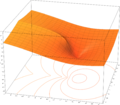  z = |W₀(x + iy)|
• 
  Superimposition of the previous three plots

Numerical evaluation

The W function may be approximated using Newton's method, with successive approximations to w = W(z) (so z = we^w) being

${\displaystyle w_{j+1}=w_{j}-{\frac {w_{j}e^{w_{j}}-z}{e^{w_{j}}+w_{j}e^{w_{j}}}}.}$

The W function may also be approximated using Halley's method,

${\displaystyle w_{j+1}=w_{j}-{\frac {w_{j}e^{w_{j}}-z}{e^{w_{j}}\left(w_{j}+1\right)-{\dfrac {\left(w_{j}+2\right)\left(w_{j}e^{w_{j}}-z\right)}{2w_{j}+2}}}}}$

given in Corless et al.^[3] to compute W.

For real ${\displaystyle x\geq -1/e}$, it may be approximated by the quadratic-rate recursive formula of R. Iacono and J.P. Boyd:^[12]

${\displaystyle w_{n+1}(x)={\frac {w_{n}(x)}{1+w_{n}(x)}}\left(1+\log \left({\frac {x}{w_{n}(x)}}\right)\right).}$

Lajos Lóczi proves^[54] that by using this iteration with an appropriate starting value ${\displaystyle w_{0}(x)}$,

• For the principal branch ${\displaystyle W_{0}:}$
  • if ${\displaystyle x\in (e,\infty )}$: ${\displaystyle w_{0}(x)=\log(x)-\log(\log(x)),}$
  • if ${\displaystyle x\in (0,e):}$ ${\displaystyle w_{0}(x)=x/e,}$
  • if ${\displaystyle x\in (-1/e,0):}$ ${\displaystyle w_{0}(x)={\frac {ex\log(1+{\sqrt {1+ex}})}{1+ex+{\sqrt {1+ex}}}},}$
• For the branch ${\displaystyle W_{-1}:}$
  • if ${\displaystyle x\in (-1/4,0):}$ ${\displaystyle w_{0}(x)=\log(-x)-\log(-\log(-x)),}$
  • if ${\displaystyle x\in (-1/e,-1/4]:}$ ${\displaystyle w_{0}(x)=-1-{\sqrt {2}}{\sqrt {1+ex}},}$

one can determine the maximum number of iteration steps in advance for any precision:

• if ${\displaystyle x\in (e,\infty )}$ (Theorem 2.4): ${\displaystyle 0<W_{0}(x)-w_{n}(x)<\left(\log(1+1/e)\right)^{2^{n}},}$
• if ${\displaystyle x\in (0,e)}$ (Theorem 2.9): ${\displaystyle 0<W_{0}(x)-w_{n}(x)<{\frac {\left(1-1/e\right)^{2^{n}-1}}{5}},}$
• if ${\displaystyle x\in (-1/e,0):}$
  • for the principal branch ${\displaystyle W_{0}}$ (Theorem 2.17): ${\displaystyle 0<w_{n}(x)-W_{0}(x)<\left(1/10\right)^{2^{n}},}$
  • for the branch ${\displaystyle W_{-1}}$(Theorem 2.23): ${\displaystyle 0<W_{-1}(x)-w_{n}(x)<\left(1/2\right)^{2^{n}}.}$

Software

The Lambert W function is implemented as LambertW in Maple,^[55] lambertw in GP (and glambertW in PARI), lambertw in Matlab,^[56] also lambertw in Octave with the specfun package, as lambert_w in Maxima,^[57] as ProductLog (with a silent alias LambertW) in Mathematica,^[58] as lambertw in Python scipy's special function package,^[59] as LambertW in Perl's ntheory module,^[60] and as gsl_sf_lambert_W0, gsl_sf_lambert_Wm1 functions in the special functions section of the GNU Scientific Library (GSL). In the Boost C++ libraries, the calls are lambert_w0, lambert_wm1, lambert_w0_prime, and lambert_wm1_prime. In R, the Lambert W function is implemented as the lambertW0 and lambertWm1 functions in the lamW package.^[61]

C++ code for all the branches of the complex Lambert W function is available on the homepage of István Mező.^[62]

See also

• Wright omega function
• Lambert's trinomial equation
• Lagrange inversion theorem
• Experimental mathematics
• Holstein–Herring method
• R = T model
• Ross' π lemma

Notes

References

• Corless, R.; Gonnet, G.; Hare, D.; Jeffrey, D.; Knuth, Donald (1996). "On the Lambert W function" (PDF). Advances in Computational Mathematics. 5: 329–359. arXiv:1809.07369. doi:10.1007/BF02124750. ISSN 1019-7168. S2CID 29028411. Archived from the original (PDF) on 2010-12-14. Retrieved 2007-03-10.
• Chapeau-Blondeau, F.; Monir, A. (2002). "Evaluation of the Lambert W Function and Application to Generation of Generalized Gaussian Noise With Exponent 1/2" (PDF). IEEE Trans. Signal Process. 50 (9). doi:10.1109/TSP.2002.801912. Archived from the original (PDF) on 2012-03-28. Retrieved 2004-03-10.
• Francis; et al. (2000). "Quantitative General Theory for Periodic Breathing". Circulation. 102 (18): 2214–21. CiteSeerX 10.1.1.505.7194. doi:10.1161/01.cir.102.18.2214. PMID 11056095. S2CID 14410926. (Lambert function is used to solve delay-differential dynamics in human disease.)
• Hayes, B. (2005). "Why W?" (PDF). American Scientist. 93 (2): 104–108. doi:10.1511/2005.2.104. Archived (PDF) from the original on 2022-10-10.
• Roy, R.; Olver, F. W. J. (2010), "Lambert W function", in Olver, Frank W. J.; Lozier, Daniel M.; Boisvert, Ronald F.; Clark, Charles W. (eds.), NIST Handbook of Mathematical Functions, Cambridge University Press, ISBN 978-0-521-19225-5, MR 2723248.
• Stewart, Seán M. (2005). "A New Elementary Function for Our Curricula?" (PDF). Australian Senior Mathematics Journal. 19 (2): 8–26. ISSN 0819-4564. Archived (PDF) from the original on 2022-10-10.
• Veberic, D., "Having Fun with Lambert W(x) Function" arXiv:1003.1628 (2010); Veberic, D. (2012). "Lambert W function for applications in physics". Computer Physics Communications. 183 (12): 2622–2628. arXiv:1209.0735. Bibcode:2012CoPhC.183.2622V. doi:10.1016/j.cpc.2012.07.008. S2CID 315088.
• Chatzigeorgiou, I. (2013). "Bounds on the Lambert function and their Application to the Outage Analysis of User Cooperation". IEEE Communications Letters. 17 (8): 1505–1508. arXiv:1601.04895. doi:10.1109/LCOMM.2013.070113.130972. S2CID 10062685.

External links

• National Institute of Science and Technology Digital Library – Lambert W
• MathWorld – Lambert W-Function
• Computing the Lambert W function
• Corless et al. Notes about Lambert W research
• GPL C++ implementation with Halley's and Fritsch's iteration.
• Special Functions of the GNU Scientific Library – GSL
• [3]